Manav Goyal

Regression Analysis - Machine Learning

Regression Analysis
Linear Regression
Logistic Regression
Regularization
Support Vector Machine (SVM)
Decision Tree
Ensemble Learning
Clustering
KNN (K Nearest Neighbours)

Regression Analysis

Basic
- Find relationship between D & I
- Dependent (D) & Independent (I) Variable
  - Dependent (Labels) => Dependent on some factor to get the output
  - Independent (Features) => Affects dependent variable
- Outliners
  - Odd one out, Extremities
- Multicollinearity
  - Independent variables are correlated with each other
  - Independent variables have Non-linear relationship
Overfitting & Underfitting
- Overfitting => Due to excess knowledge of attributes, Model tries to use all attributes (even the least important ones)
  - Resampling => Using random training data, many number of times
  - Holding a Validation dataset => Separating some data from training data for checking Overfitting
- Underfitting => Due to lack of enough attributes, Model doesn't has enough knowledge and gives incoherent results
Types
- Linear Regression
- Logistic (Logit) Regression

Linear Regression

Dependent variable is continuous in nature
Linear relationship between I & D
Simple Linear Regression
- If 1 DV & 1 IV
- Equation => y = α_o + α₁x₁ = mx + c
  - y => Dependent variable, log of odds
  - x => Independent variable
  - α => Regression coefficient => Represents the importance of that feature
  - m => weights
  - c => bias or intercept
- Best Fit Line
  - Line obtained as output from the model
  - If actual & predicted values are close then it is a good fit line
- Solve
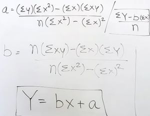
  - Predict value of "Y" for a given value of "X", Find Error
- Code
```
    from sklearn.linear_model import LinearRegression
    x = data[["val1"]] # Independent variable
    y = data["val2"] # Dependent variable
    reg = LinearRegression()
    reg.fit(x, y) # Creates the model
    reg.predict([[value]]) # Predicts the value
    print(reg.coef_) # Slope of line
    print(reg.intercept_) # Intercept of line
```

Multiple linear regression

If 1 DV & IV > 1
Equation => y = α_o + α₁x₁ + ... + α_mx_m

Code

    from sklearn.model_selection import train_test_split
    from sklearn.linear_model import LinearRegression
    x = data[["val1", "val2"]] # Independent variables
    y = data["val3"] # Dependent variable
    x_train, x_test, y_train, y_test = train_test_split(x, y, test_size=0.3, random_state=10) # Splitting data
    reg = LinearRegression()
    reg.fit(x_train, y_train) # Creates the model using training data
    reg.predict(x_test) # Predicts the value
    reg.predict([[val1, val2]]) # Predicts the value
    reg.score(x_test, y_test) # Predicts the score of the model

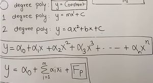
Polynomial regression
- Using linear regression for non-linear dataset

Logistic Regression

Dependent variable is binary (Categorical)
1 (True, Success), 2 (False, Failure)
Independent variable can be continuous or binary
Deals with probability to measure the relationship between dependent & independent variables
Sigmoid Equation => Y = 1/1 + e^-x
- Converts the IV into an expression of probability w.r.t DV
0.5 is taken as middle value and points on it are considered as Unclassfied
Dataset should be free of missing values
- 60-100 data points for each output
Cost Function/Log Loss = -y * log(Y) - (1-y) * log(1-Y)
- To find global minima

Code

    from sklearn.model_selection import train_test_split
    from sklearn.linear_model import LogisticRegression
    x = data[["val1"]] # Independent variables
    y = data["val3"] # Dependent variable
    x_train, x_test, y_train, y_test = train_test_split(x, y, test_size=0.3, random_state=10) # Splitting data
    reg = LogisticRegression()
    reg.fit(x_train, y_train) # Creates the model using training data
    reg.predict(x_test) # Predicts the value
    reg.score(x_test, y_test) # Predicts the score of the model

Applications
- Fraud detection
- Disease diagnosis
- Emergency detection
- Spam email detection

Regularization

Basic
- Shrink the magnitude of the regression coefficient and reduce the complexity of model
Ridge regression
- Ridge (R) = Loss + α||W||² (Penalty)
- Loss = Different between the predicted and actual value
- W is vector of coefficients = Sum of squares of all coefficients
- Magnitude of coefficients decreases with increase in value of α
- Used when multicollinearity between independent variables
Lasso regression
- Ridge (R) = Loss + α||W|| (Penalty)
- W = Sum of absolute values of all coefficients
- Magnitude of coefficients decreases till 0 with increase in value of α => Acts as feature selection
Elastic net regression
- Ridge (R) = Loss + α₁||W||² + α₂||W||

Support Vector Machine (SVM)

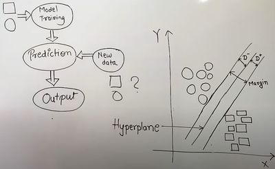
Decision Boundary (Hyperplane)
- Boundary that decides if that new data belongs to which class
- Maximum Margin Hyperplane (MMH)
  - Hyperplane with greater Margin should be selected
  - It is better for future prediction and reduces Misclassification which reduces Error rate
Margin = D^- + D⁺
Support Vectors
- The two points that are closest to the Hyperplane along which lines are drawn
Linearly Separable Data
- When data points can be separated by drawing a single line
Non-linear Separable Data
- When data points can't be separated by drawing a single line
- Kernel Function
  - Takes low dimensional feature space as input and gives high dimensional feature space as output

Decision Tree

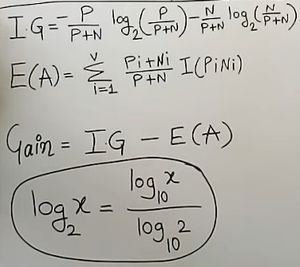
Select target attribute
Find IG of target attribute
Find Entropy of rest of the attributes
Calculate Gain and attribute with maximum gain will be the root node of DT
If the value of attribute of root node belongs to only one value then put that value as child node otherwise take the next node with next highest Gain value

Ensemble Learning

Ensemble learning works well when different models make independent mistakes
Base Learners
- Heterogeneous Ensemble
  - Using different algorithms to train
- Weak Learners
  - Using different training sets to train
  - Combining all these weak classifiers/models will generate a strong classifier
Methods
- Bagging (Bootstrap Aggregation)
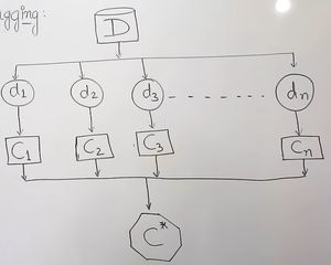
  - Parallel ensemble method
  - "D" is original training data
  - Bootstrap Samples (d) is data set obtained by randomly selecting samples with replacement from D
  - Classifiers (c) is trained using "d"
  - Final strong ensemble classifier is obtained by combining all the obtained classifiers
    - Uses Voting mechanism to predict the output
- Boosting
  - Sequential ensemble method, Can increase over-fitting
  - Training data (D) contains instances/records/tuples/samples along with their weights which are initially assumed to be equal
  - Random instances are selected to train first classifier/model
  - Now all instances are given as input to this classifier and weights of the instances are increased for next model selection whose classification is done wrong
  - Train a new model and repeat the previous step
  - Combine all models to create a final strong model which uses voting mechanism to predict the output
Voting Classifier
- Hard (Majority) Voting
  - Final result is mode of outputs of all classifiers
- Soft Voting
  - Predictive probability => Probability of being from all the classes
  - Calculate average of probabilities of all classifiers w.r.t that particular class
  - Maximum probability of class will be the final result
Random Frost
- Kind of ensemble classifier which uses decision trees in randomized way
- Original Dataset (OD) is training data
- Create a Bootstrap Dataset (BD) by randomly selecting from OD, Duplication is allowed
- Construct a Decision Tree by randomly selecting subset of variables and choosing the better of them for creating a node
- Voting mechanism is used for selecting the final output out of all the results obtained from decision tress for a test data

Clustering

DBSCAN (Density based spatial clustering of applications with noise)
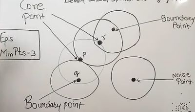
- Epsilon (Eps) is Radius of circle
- Minimum Points is the number of points inside the circle
- Core point is the point from which if a circle is created will contain at least minimum points
- Boundary point is a point which is neighbor of core point but does not satisfy the minimum point criteria
- Noise point (Outlier) is the point which are none of the above two points
- Directly density reachable
  - Point must be a neighbor of point "P"
  - Point "P" must be a core point
  - Then the point is directly density reachable from point "P"

K-means Clustering

Make 2 centroids by selecting the first 2 points
Calculate Euclidean distance of next row from both centroids, The one with less distance with be its cluster
Calculate new centroid = (Old centroid + new value / 2) and repeat the previous step

Code

    from sklearn.cluster import KMeans
    from sklearn.preprocessing import MinMaxScaler
    from matplotlib import pyplot as plt
    scaler = MinMaxScaler()
    scaler.fit(data[["val1"]])
    data["val1"] = scaler.transform(data[["val1"]])
    scaler.fit(data[["val2"]])
    data["val2"] = scaler.transform(data[["val2"]])
    plt.scatter(data.val1, data.val2)
    km = KMeans(n_clusters=N) # "N" will be equal to the number of clusters observed
    predicted = km.fit_predict(data[["val1", "val2"]])
    data["cluster"] = predicted
    data1 = data[data.cluster=0]
    data2 = data[data.cluster=1]
    dataN = data[data.cluster=N]
    plt.scatter(data1.val1, data1.val2, color="green")
    plt.scatter(data2.val1, data2.val2, color="red")
    plt.scatter(dataN.val1, dataN.val2, color="blue")
    km.cluster_centers_
    plt.scatter(km.cluster_centers_[:,0], km.cluster_centers_[:,1], color="black", marker="*") # Plot centroid values
    plt.xlabel("val1")
    plt.ylabel("val2")
    plt.plot()

Hierarchical Clustering
- Agglomerative Clustering
  - Start with individual data points and start making clusters
  - Bottom to Up approach to form a Dendrogram
  - Single Linkage
    - Create a distance matrix, Diagonal elements will be 0
    - Find the smallest value and cluster those 2 points
    - Create a distance matrix, Distance with cluster will be taken as minimum of all distance with points and repeat the previous step
  - Complete Linkage
    - Distance with cluster will be taken as maximum of all distance with points
- Divisive Clustering
  - Start with a complete cluster consisting of all points and divide them
  - Top to Down approach to form a Dendrogram

KNN (K Nearest Neighbours)

Classifies the objects based on the closest training examples
K is number of nearest neighbors