Image Enhancement - Image Processing
- Spatial and Frequency domain
- Image Enhancement Methods
- The principal objective of enhancement is to process an images so that the result is more suitable than the original image for a SPECIFIC application
- Uses
- Highlighting interesting details in the images
- Removing noise from the images
- Making images more visually appealing
- Enhance hidden information
- Filter important image features
- Discard unimportant image features
- Types
- Spatial Domain Methods (Image Plane)
- Techniques are based on direct manipulation of pixels in an image
- Methods
- Point Processing
- s = T(r)
- Gray-Level Transformation Function
- Types
- Contrast stretching
- Thresholding
- Basic Gray Level Transformation
- log, nth root, identity, nth power, inverse log
- Digital/Image Negative
- It is useful when for enhancing white details embedded in dark regions of the image
- S = L-1-r
- r = pixel value of given image
- L = grey-level value
- 256 for 8-bit per pixel image
- Log Transformations
- Expands the details of darker regions in an image
- s = c * log(1+r)
- Power-Law Transformations
- Piecewise-Linear Transformation Functions
- Arbitrarily complex
- More user input
- Type of Transformations
- Contrast stretching
- Increase the dynamic range of the gray levels in the image
- S = r - c[b-a/d-c] + a
- a = s1, b = s2, c = r1, d = r2
- Causes for poor image
- Poor illumination
- Wrong lens aperture
- Wrong shutter speed
- Lack of dynamic range in the imaging sensor
- Gray-level slicing
- Highlighting a specific range of gray levels in an image
- Bit-plane slicing
- It divides the image into bit planes on the basis of contribution of each bit in the image
- Steps
- Convert each pixel into binary
- Create "n" planes where "n" is number of bits
- Fill first plane by taking first bit of each binary and so on
- Mask Processing
- Frequency Domain Methods
- Techniques are based on modifying the Fourier transform of the image
- Combination Methods
- There are some enhancement techniques based on various combinations of methods from the first two categories
- Histogram processing
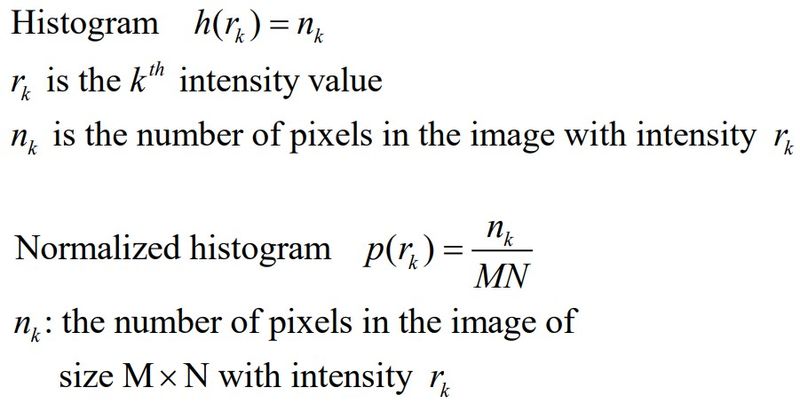
- Histogram Equalization
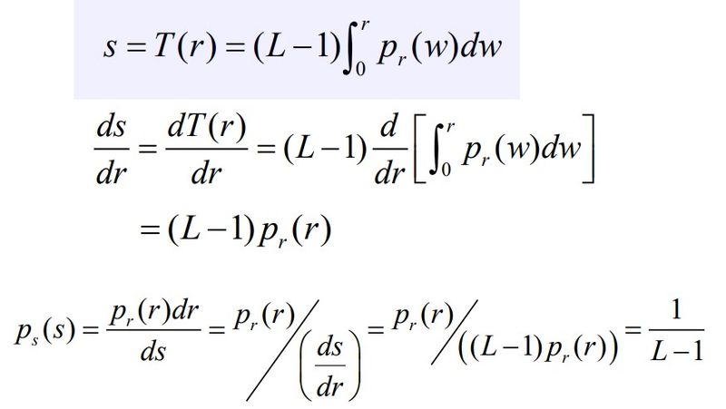
- The intensity levels in an image may be viewed as random variables in the interval [0, L-1]
- Let pr(r) and ps(s) denote the probability density function (PDF) of random variables "r" and "s"
- s = T(r), 0 ≤ r ≤ L-1
- T(r) is a strictly monotonically increasing function, one-to-one mapping, continuous and differentiable
- 0 ≤ T(r) ≤ L-1 for 0 ≤ r ≤ L-1
- ps(s)ds = pr(s)dr
- Steps
 - If grey level is not given directly then Take maximum value > Represent it in power of 2 > Take that as L
- Create table for new Grey level (Equal to histogram equalization level obtained from previous table) & No. of Pixel
- Plot histogram and calculate Output image
- Spatial Filtering
- Used to Smoothing and Sharpening of images by removing very High/Low frequency components
- Spatial filtering is defined by
- A neighborhood
- An operation that is performed on the pixels inside the neighborhood
- Types in Frequency Domain
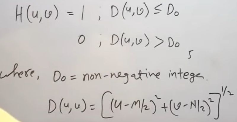
- Low pass (preserve low frequencies)
- Remove High frequency components, Keeps Low frequency
- Used to Smoothen the image
- Removes noise (as noise is mostly High frequency)
- Types and their Transformation function
- Ideal low Pass
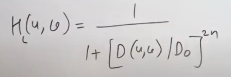
- Butterworth low Pass
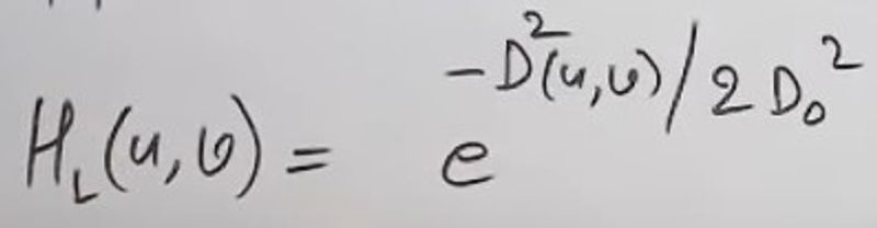
- Gaussian low Pass
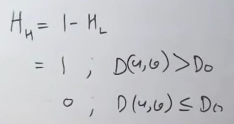
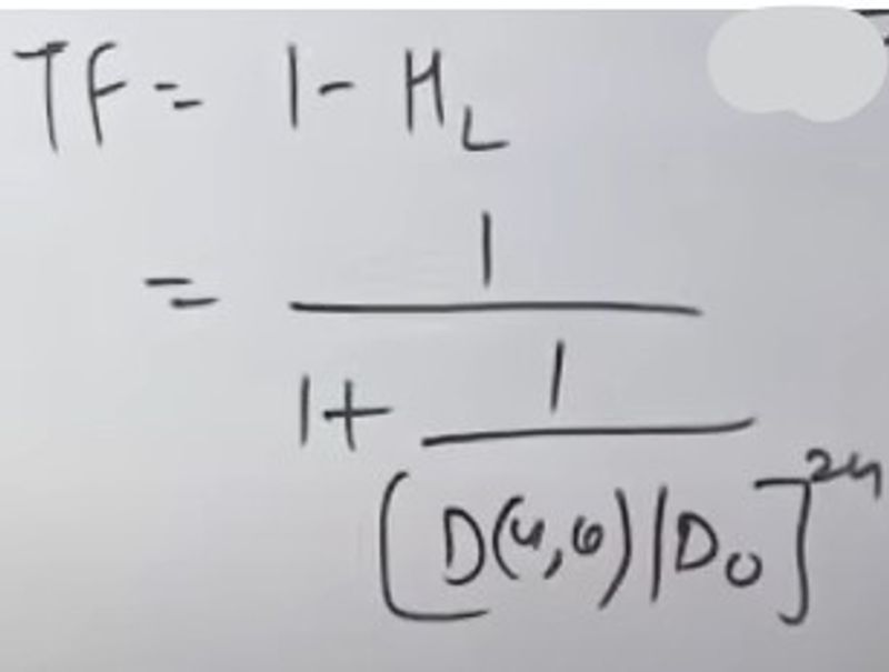
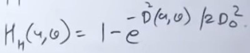
- High pass (preserve high frequencies)
- Remove Low frequency components, Keeps High frequency
- Used to Sharpen the image
- No background
- Types
- Ideal low Pass
- Butterworth low Pass
- Gaussian low Pass
- Band-pass (preserve frequencies within a band)
- Band-reject (reject frequencies within a band)
- Spatial Filtering Methods
- Linear
- A filtering method is linear when the output is a weighted sum of the input pixels
- T[a1f1(t,z) + a2f2(t,z)] = a1T[f1(t,z)] + a2T[f2(t,z)]
- Linear Spatial Filtering Methods
- Correlation
- Often used in applications where we need to measure the similarity between images or parts of images (Pattern matching)

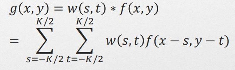
- Convolution
- Similar to correlation except that the mask is first flipped both horizontally and vertically
- If symmetric, w(s,t) = w(-s,-t), then convolution is equivalent to correlation
- Non-Linear
- Steps for Filtering in the Frequency Domain
- Take image f(x,y) of dimension MxN
- Give padding to form fp(x,y) of dimension PxQ, where P = 2M and Q = 2N
- Zero Padding
- Replicate Edge Pixels
- Wrap Around Edge Pixels
- To centralize image multiply
- Filter is H(u,v), Fourier transform the image F(x,y)
- Find inverse of DFT
- g(x,y) = T-1[g(u,v)] (-1)x+y
- Steps for Filtering in the Spatial Domain
- Slower than Frequency Domain
- Convolution is used
- Statistical Order/Non-Linear Filters
- Mean Filter
- Weighted Average Filter
- Weighted Matrix * Elements/Sum of all Elements
- In Weighted Matrix we gave more weight to the center value
- Take centre value of filter as whatever value you want and others as 1
- Median Filter
- Sometimes a median filter works better than an averaging filter
- Min Filter
- Max Filter
- Smoothening Spatial Filters
- Useful in removing noise from images, Highlighting gross detail
- Blurring -=> Pixel Averaging
- Types
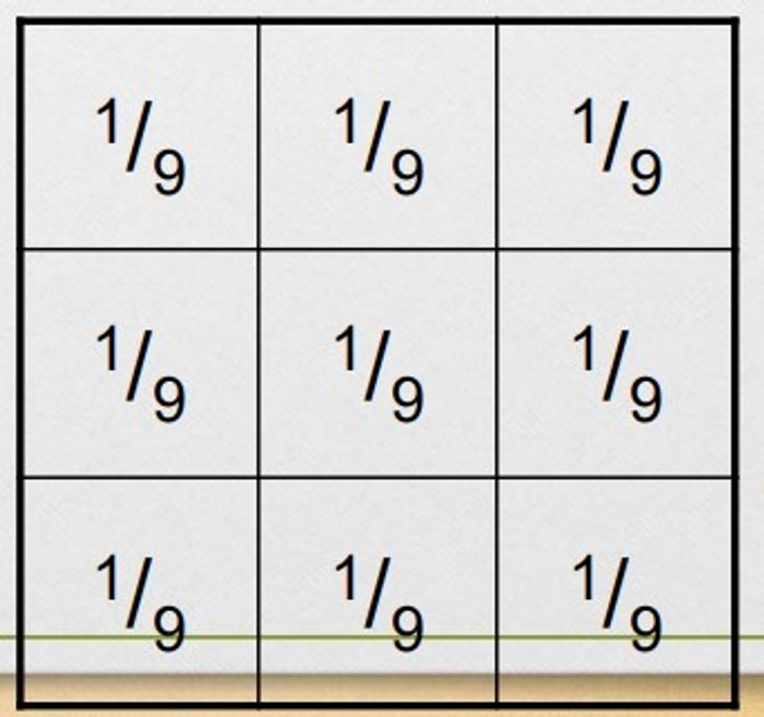
- Simple averaging filter
- Average all of the pixels in a neighborhood around a central value
- Sum of all Elements/Total number of elements
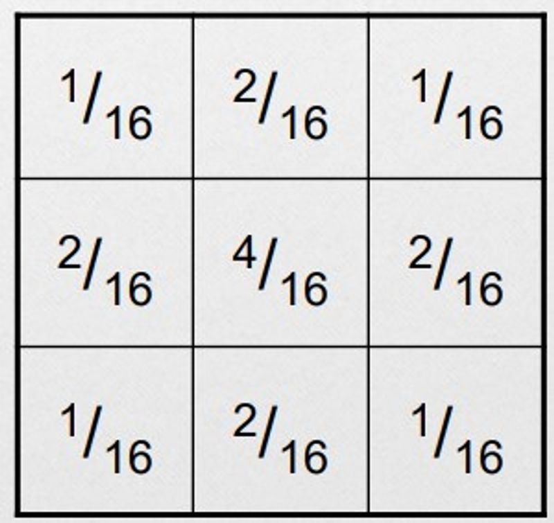
- Weighted Smoothing Filters
- Pixels closer to the central pixel are more important
- Approaches to dealing with missing edge pixels
- Omit missing pixels
- Only works with some filters
- Can add extra code and slow down processing
- Pad the image
- Typically with either all white or all black pixels
- Replicate border pixels
- Truncate the image
- Allow pixels wrap around the image
- Can cause some strange image artifacts
- Sharpening Spatial Filters
- Sharpening spatial filters seek to highlight fine detail based on spatial differentiation
- Remove blurring from images
- Highlight edges
- Applications
- Electronic Printing, Medical imaging, Industrial inspections, Autonomous guidance
- Spatial Differentiation
- Differentiation measures the rate of change of a function
- Requirements for digital derivative
- First derivative
- Must be zero in flat segment
- Must be nonzero along ramps
- Must be nonzero at the onset of a gray-level step or ramp
- 1st Derivative -=> f(x+1) - f(x)
- Second derivative
- Must be zero in flat segment
- Must be zero along ramps
- Must be nonzero at the onset and end of a gray-level step or ramp
- 2nd Derivative -=> f(x+1) - f(x-1) - 2f(x)
- Comparing the response between first- and second-ordered derivatives
- First-order derivative produce thicker edge
- Second-order derivative have a stronger response to fine detail, such as thin lines and isolated points
- First-order derivatives generally have a stronger response to a gray-level step
- Second-order derivatives produce a double response at step changes in gray level
- In general the second derivative is better than the first derivative for image enhancement
- The principle use of first derivative is for edge extraction
- Sharpening Filters
- Laplacian Image Enhancement
- Isotropic
- One of the simplest sharpening filters
- We will look at a digital implementation
- Steps
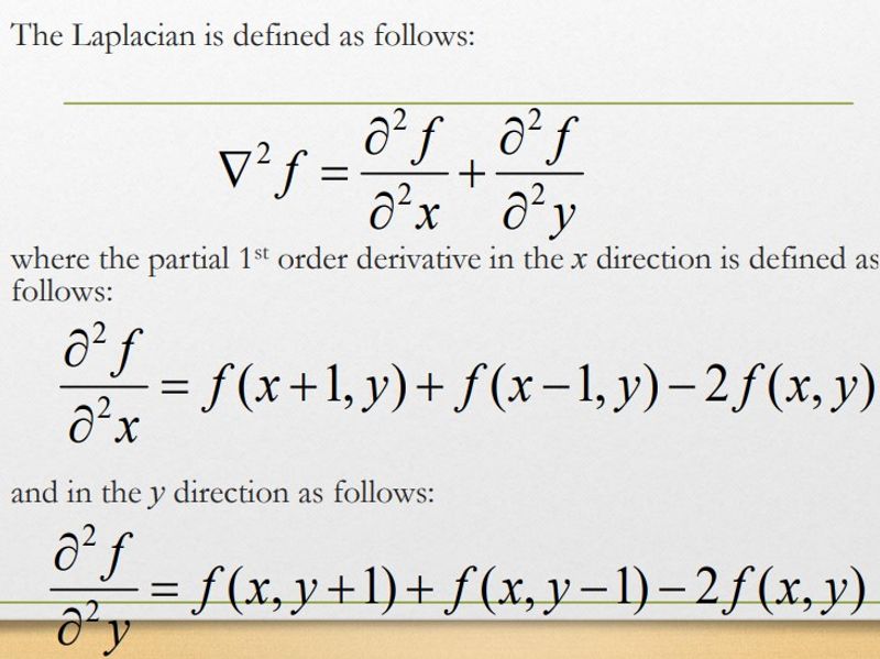
- Subtract the Laplacian result from the original image to generate our final sharpened enhanced image
- Variant
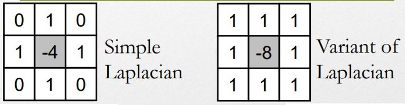
- Enhanced Laplacian filter -=> Add 1 in the middle pixel
- Use of First Derivative for Edge Extraction
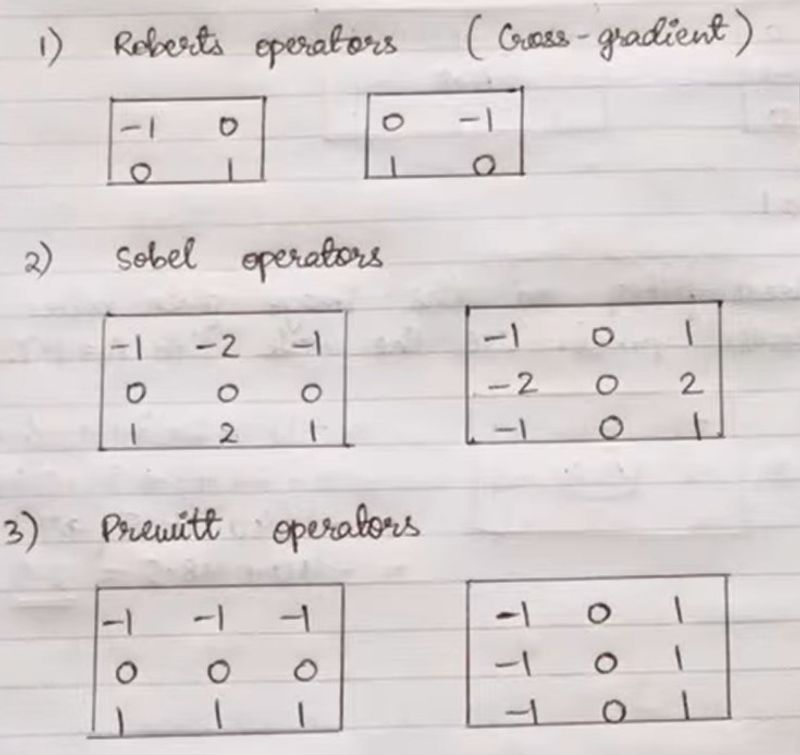
- Roberts operator (Cross gradient)
- Roberts cross operator
- Prewitt operator
- Sobel operator
- Zero crossing property of Laplacian filter
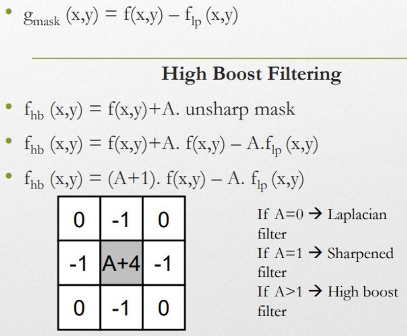
- Un-sharp Masking
- Primarily used in the printing and publishing industry to sharpen images
- Process of subtracting an un-sharp (smoothed) version of image from the original
- Blur the original image
- Subtract the blurred image from the original (Result is called mask)
- Sharpened = Original - Blurred image
- Add the mask to the original
- Discrete Fourier Transform

- N is number of values
- k is from 0 to N-1
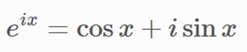
- In Continuous Fourier Transform, don't divide by N
- Convert filter from
- Spatial to Frequency
- Fourier Transform
- Take average of points, g(x,y)
- G(u,v) = H(u,v) * F(x,y) = Filter * Image
- Frequency to Spatial
- Inverse Fourier Transform
- Homomorphic Filtering
- f(x,y) is categorized by
- Illumination
- Light falling on the object
- Reflectance
- Light reflecting from the object
- Approach is to separate illumination and reflectance components
- f(x,y) = i(x,y) * r(x,y)
- F(u,v) ≠ F(i(x,y) * r(x,y)) -=> Fourier transform is not possible directly
- Z(x,y) = ln(f(x,y))
- Z(u,v) = Fi(u,v) + Fr(u,v) -=> Transform of Z(x,y)
- Fi(u,v) = F[ln(i(x,y))]
- Fr(u,v) = F[ln(r(x,y))]
- S(u,v) = Z(u,v) * H(u,v)