Primary focus of Regional characteristics -=> Color, Texture
Texture
Texture is characterized by the relationship of the intensities of neighboring pixels ignoring their color, Texture provides information in the spatial arrangement of colors or intensities in an image, Texture is a repeating pattern of local variations in image intensity, Can't be defined for a point, Texture is characterized by the spatial distribution of intensity levels in a neighborhood
Uses -=> Surface inspection, Scene classification, Surface orientation, Shape determination
Feature Vector -=> Set of quantitative measure of the arrangement of intensities in a region
Extracting Textural Features
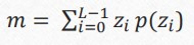
Statistical methods -=> Texture of regions in an image through higher order moments of their gray-scale histograms
Gray Level Histogram
Features
Mean -=> The average gray level of each region and it is useful only as a rough idea of intensity not really texture
Variance -=> The amount of gray level fluctuations from the mean gray level value
Skewness -=> Measure of the asymmetry of the gray levels around the sample mean -=> If skewness is negative, the data are spread out more to the left of the mean than to the right
Kurtosis -=> Measure of how outlier-prone a distribution is, Describes the shape of the tail of the histogram
Gray Level Co-occurrence Matrix (GLCM) -=> Use of second-order statistics of the gray-scale image histograms, A second-order probability is often called a GLC probability
Features
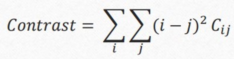
Inertia (Contrast) -=> Element difference moment of order 2, which has a relatively low value when the high values of C are near the main diagonal
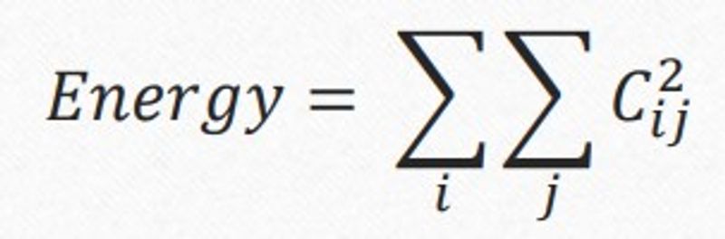
Energy -=> Highest when all values in the co-occurrence matrix are all equal
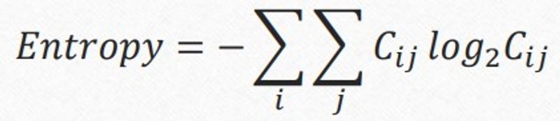
Entropy -=> The measure of randomness of the image gray levels
Absolute Value
Inverse Difference
Steps
No. of Gray-Levels (N), Direction of Pair (θ)
Construct a NxN matrix, Values equal to the number of Pairs of (i,j) in θ direction
Divide the matrix by number of total Pairs to Normalize
Structural methods -=> Texture as the composition of well defined texture elements such as regularly spaced parallel lines
Model based methods -=> Generate an empirical model of each pixel in the image based on a weighted average of the pixel intensities in its neighborhood
Transform-based methods -=> Convert the image into a new form using the spatial frequency properties of the pixel intensity variations
Local Binary Pattern (LBP)
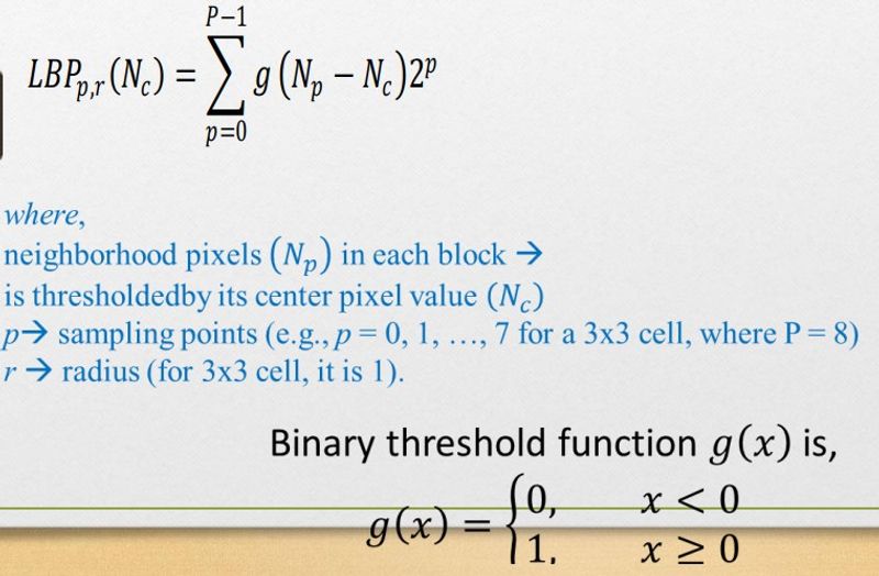
Simple yet very efficient texture operator which labels the pixels of an image by thresholding the neighborhood of each pixel and considers the result as a binary number
Steps
Divide the examined window to cells
For each pixel in a cell, compare the pixel to each of its 8 neighbors
Follow the pixels along a circle -=> Clockwise or Counter-clockwise
Where the center pixel's value is greater than the neighbor, write "1", Otherwise, write "0"
This gives an 8-digit binary number (which is usually converted to decimal for convenience)
Compute the histogram, over the cell, of the frequency of each "number" occurring
Extract Binary code generated and Convert in Decimal number